Prelab
Before lab, take two pictures, with the camera lense at the same position, but pointing in slightly different directions. Try get at least a 50-80% overlap between the images. It is best if you take the pictures in a large area, since this will reduce the difficulties coming from taking a picture from multiple positions. Here is an example, although do be sure to take some pictures with more overlap than this. (They will be useful in later labs.)
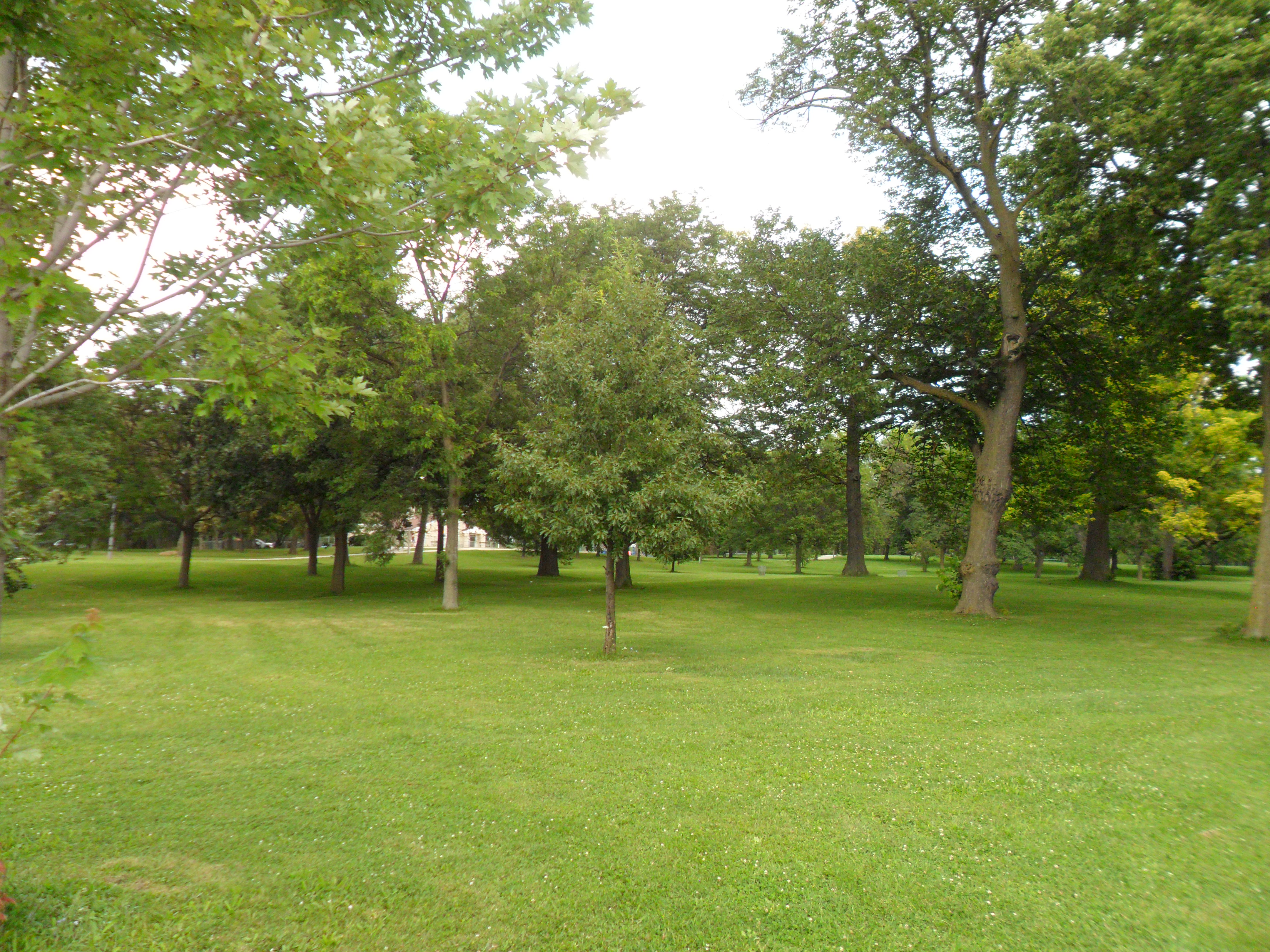
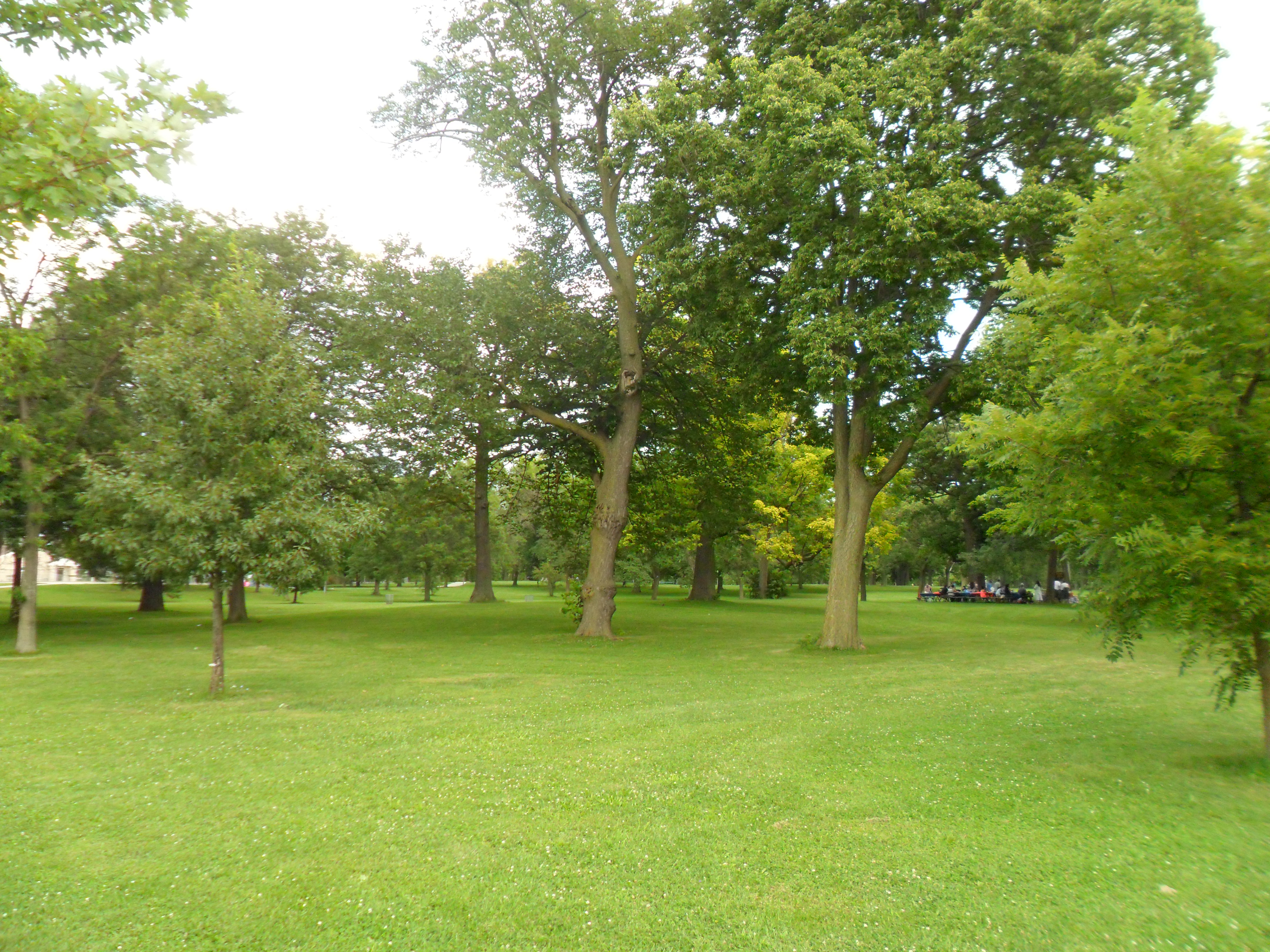
A key concept for this lab is that two pictures taken from the exact same position only have image-based warping between them, not any 3D effects. In some sense, what the camera sees when it rotates around its center is a large flat image. We can map between any two images taken from the same position using a full 8-DOF homography, the same transform we can use to map a picture of a flat object from one camera view to another. In this lab, we will stitch two pictures taken from a single point of view together by finding a homography between the two pictures.
Many cameras today have multi-megapixel images. In their uncompressed form, these images are very large. Since we usually maintain several copies of an image in matlab, this can easily fill your computer's memory. I recommend reducing the size of these images until Matlab does not warn you that they are too large to display on your screen when you run imshow
Deliverables
- Zip code of your source code for this lab. This should contain a zipped folder named "lab2" which contains the m-files directly inside it. Please do not include any additional folders inside the lab2 folder.
transformImage.mmakeASmall.mmakeA.mmakeB.mfindTransform.mstitch.m- your top-level script- Your stitched results image.
In all your source files, be sure to include your name and the quarter (e.g. Winter 2012-2013. And, in the templates you copy from below, be sure to edit the author block that follows the help block so that it is accurate for you.
Useful Matlab commands for this lab
- ndgrid
- Create a set of n-dimensional grids with the values of the index for each point in the grid. e.g.
[ii,jj,kk] = ndgrid(1:2,1:3,1:4); - hold on
- Keep the currents contents of a graph. The next plot will be plotted on top. e.g.
hold on - hold off
- Opposite of hold on.
- plot
- Plot 2-d data. e.g.
plot(jj,ii,'ro-'). If you usedocfor help, be sure to check out the LineSpec link. - repmat
- and friends frpom below
- imfuse
- Overaly two images with 0.5 alpha compositing. e.g.
IFused = imfuse(I1,I2,'blend');
Homographic point transforms
As discussed in class, you can compute many useful warpings using matrix multiplication.
For example, you can rotate a point counter-clockise by multiplying it by the matrix
  [inew] = [cos(theta), -sin(theta)] [iold]
  [jnew]   [sin(theta),  cos(theta)] [jold]
Which we can represent in short form as
inew = R iold
Or, using homographies, we can do a full projective homography from one 2D image to another using
  [inew] = [1+h1,1,   h1,2, h1,3] [iold]
  [jnew]   [  h2,1, 1+h2,2, h2,3] [jold]
  [wnew]   [  h3,1,   h3,2, 1   ] [1   ]
In the formula above, I have replaced some elements with ones (1's) that we can force to be one (1) without changing the meaning of the resulting homography. (Recall that if all of i, j, and w are multiplied by the same scaling factor, it is still the same point.) Again, we can represent this simply as
̃inew = H ̃iold
You can find a table of homographies in the text at Table 2.1 (p. 35/)
Create a grid of points using ndgrid. Plot this grid on top of your first image using hold on and plot commands.
Now transform this grid using a rotation, translation, or any other transform you would like to try. Plot the points over a blank destination image.
Transforming the image
Once you are able to transform points, you can move on to transforming an image. You can start by transforming an image in your top-level script, then cut (not copy) your code and paste it into an m-file using the template below.
The most natural way to transform an image is, for each pixel in the original image, to compute the indices of the corresponding pixel in the new image, and then color that pixel the same color as the original image -- in other words, to project the original image onto the new transformed iamge. However, in practice, this can result in some pixels in transformed image not getting any color at all, even though they are inside the transformed area. If you are enlarging an image, this approach will produce scattered individual dots of color wherever a pixel lands.
Instead, we transform the pixel indices from the destination image back into the original space, and copy the color from there into the new image.
You can do this using a for-loop, or, if you prefer, using image indexing and resizing. If you choose the indexing route, you might be able to obtain faster results (though this approach can be memory-bound if you use large images). This technique requires a variety of methods:
- Flattening an array with x(:)
reshapesub2indind2sub- multiplying by
ones(x,k), e.g.h'*ones(1,5)will repeat the columnh'five times. repmat, although I have found the ones trick above to be faster.- Concatenating matrices, e.g.
[a,b;c,d]or equivelently,[a b;c d]
There are lots of fun tricks you can play with these methods. In particular, you can assign to a square region from a column vector (or vise-versa) if they both have the same size:
x = zeros(4,5);
x(:) = 1:prod(size(x));
When you map the pixel locations, they most often will not fall exactly on a pixel in the source image. Just round to the nearest pixel, and use the value of that pixel.
After you have mapped the image onto a black background, you can composite it with another image using imfuse(I1,I2,'blend');
Once you are able to successfully apply a transformation to an image, wrap your result into a method meeting this description: (You can copy-paste this from chrome or Firefox into your m-file. Matlab should automatically pick up the name of the m-file when you save it.) Save the m-file in the same directory as your top-level script. This should also be your Matlab working directory. After that, you can use transformImage like any other Matlab function. You can even use help transformImage
% INew = transformImage(szDest,I1, H)
%
% Transform image I1 into an image of size szDest.
%
%  szDest -- size of the image to create (size of I2).
%  I1 -- the image to transform
%  H -- The homography supplied is from I2 to I1.
%    [i1]   [         ] [i2]
%    [j1] = [    H    ] [j2]
%    [w1]   [         ] [w2]
%
%  INew -- The transformed image, which has size szDest = size(I2), and is
%  in the coordinate frame of I2, but contains the warped image I1.

% Author: Phileas Fogg
% Term: Winter 2012-2013
% Course: CS498 - Computer Vision
% Assignment: Lab 2 - Homographic image warping

function INew = transformImage(szDest,I1, H)
Marking correspondences in an image
Using ginput, mark four points on the first image. Mark the corresponding points in the second image. That is, mark four distint points on objects in the first image, and mark the same points on the objects in the second image. Choose points that you can identify well, such as corners.
Save the points you use somewhere in your source code, so you don't have to remark the points every time you run the program. Ideally this would not be hard-coded in one of your matlab functions.
In class, we discussed a technique for solving a linear system of equations to find a homography from one point-set to another. Apply this technique as follows
Create a method, makeASmall that creates two rows of the A matrix. As in section 6.1.3 (p. 279/) of the book, this is
Asmall = [i j 1 0 0 0 -i2i -i2j]
         [0 0 0 i j 1 -j2i -j2j]
where i and j are the coordinates from the image to be mapped from and x2 and y2 are the coordinates in the image to be mapped to. (Recall two things: First, i and j correspond to j and i, in that order, unless you want your i axis to point down. Second, the point mapping is the inverse of the image mapping. You may want to compute the homograpy "backwards" from the image you want to map "to" to the image you want to map "from".)
Use this header for the makeASmall method
% ASmall = makeASmall(i1,j1,i2,j2)
%
% i1, j1 -- the indices in the first image
% i2, j2 -- the indices in the second image
%
% A -- Two rows of the A matrix with used to solve for the Homography matrix,
%         representing a single point correspondence.
%
% Note: This assumes the homography is in terms of [i j 1] instead of
% [i j 1].   ([i j 1] is the same as [j i 1]).

% Author: Phileas Fogg
% Term: Winter 2012-2013
% Course: CS498 - Computer Vision
% Assignment: Lab 2 - Homographic image warping

function ASmall = makeASmall(i1,j1,i2,j2)
Create a method that forms the full A matrix by concatenating all of the Asmall matrices for the four point correspondences to form the full A matrix. There should be 2*n rows, where n is the number of correspondences you use (n=4 is the minimum you will need).
% bigA = makeA(matches)
%
% matches -- a matrix where each row represents the indices of a match,
%            [i1 j2 i2 j2]
%
% bigA -- the full A matrix which is used to solve for the Homography matrix,
%         including all point correspondences.

% Author: Phileas Fogg
% Term: Winter 2012-2013
% Course: CS498 - Computer Vision
% Assignment: Lab 2 - Homographic image warping

function bigA = makeA(matches)
Create a method that creates the full b column vector. This vector is the concatenation of the bsmall vectors for each pair of corresponding points, where bsmall is ...
bsmall = [i2-i]
         [j2-j]
Use this header for the makeB method
% bigB = makeB(matches)
%
% matches -- a matrix where each row represents the indices of a match,
%            [i1 j2 i2 j2]
%
% bigB -- the full B matrix with used to solve for the Homography matrix,
%         including all point correspondences.

% Author: Phileas Fogg
% Term: Winter 2012-2013
% Course: CS498 - Computer Vision
% Assignment: Lab 2 - Homographic image warping

function bigB = makeB(matches)
Concatenate a stack of Bsmall matrices to form the B matrix
Solve B = A*linearH for linearH.
Reshape linearH into a square matrix. Indexed-assignment can help here. But be aware that Matlab counts along columns, whereas the linearH matrix is indexed along the rows.
You will use findTransform in some of the following labs, so be sure to write it so that it can accept more than four points. With more than four points, the problem is over-constrained, but the best solution to A linearH = b is a good first-level approximation to find the best point matches. If you use linearH = A\b to solve the system of equations, Matlab will automatically find the best solution under the hood.
Wrap all of the above into another method, findTransform, which conforms to the following heading:
% H = findTransform(matches)
%
% matches -- list of matches in rows of [i1 j1 i2 j2]
%
% H -- transformation [i2,j2,w2]' = H*[i1,j1,1]'

% Author: Phileas Fogg
% Term: Winter 2012-2013
% Course: CS498 - Computer Vision
% Assignment: Lab 2 - Homographic image warping

function H = findTransform(matches)
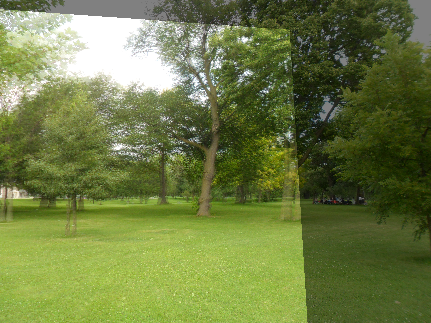
Now you can use your image transformation techniques from the first section to map one image onto another!
After fusing your two images, you should have something like this:
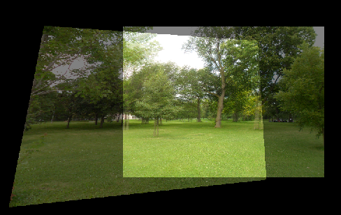
One of the fun ideas below is to modify things a bit so you get a black matted margin around the destination image:
Fun Ideas
- Try creating a black mapped area around the image, as shown in the second image above. You can either modify the transform to go from the larger image, or modify your transforming function to accept an "offset" for the origin of the iamge, which is taken into account before transforming.
- Use bilinear interpolation instead of rounding to the nearest pixel. This gives a smoother image when you enlarge.
- In game engines, "mip-maps" or image pyramids are used to avoid aliasing when shrinking an image. Try building a pyramid of down-sampled smoothed images, and automatically selecting the scale based on how many pixels the destination image pixel would cover when mapped back onto the source. (Perhaps you can reproduce these images "from scratch.")
- Try stitching several images in a row, either using homographies or panographies (6.1.2, p. 277/)
- The
imfuseapproach we take here causes the images to be darker where they don't overlap. Can you make the images have full brightness like Figure 6.5. (p. 278/) by creating your own alpha-mapping strategy? You can create a mask for the transformed image(s) by transforming an all-ones image using the same mapping function - Can you build an entire panorama, going full-circle around a point? You may want to project the images on the the surface of a cube. Could you find the homography to go from one cube surface to the next? This would probably require some full 3-D camera geometry.
- Google Street-view is built as a sequency of panoramas, centered at distinct points on a street. Can you build a simple "street view" of a pretty spot on campus?
- Do you have your own fun ideas that you would like to try?
Readings
- Szelinski (2011) Section 6.1 - 6.1.4 (pp. 275-280/)