This IS NOT a required lab for the Winter 2014-2015 offering of CS498 Computer Vision. However, you may find it handy for your final project, depending on what you decide to do.
Deliverables
- Zip code of your source code for this lab. This should contain a zipped folder which contains the m-files directly inside it. Please do not submit deeply-nested source files.
findDescriptor.mextractSamples.mextractDescriptor.mextractDescriptors.msift.m- your top-level script- Answers to these questions
- How does the SIFT feature-point descriptor achieve illumination invariance?
- How does the SIFT feature-point descriptor handle nonlinear illumination changes?
- How does the SIFT feature-point descriptor achieve rotation invariance?
- How does the SIFT feature-point descriptor achieve scale invariance?
Overview
In this lab, you will perform a few steps to extract SIFT feature-point descriptors at the interest-points you found in last week's lab.
- Compute derivatives of image (again)
- Compute principle orientation of an image point (using provided code)
- Resample the derivative patches at the desired orientation around the sample point
- Compute the histogram of gradients from the resampled patches
- Visually inspect... as a sanity check...
Compute the derivatives of the images
We are going to require the derivative images for a number of tasks in this lab. However, this time, the derivatives are of the blurred images, not the dOG images. As a first step, derivatives for every level in the stack, using this method template. But be warned -- this is the first lab where having these derivatives correct can influence your results. In particualr, dx increases with increasing j, but dy actually decreases with increasing i, since i increases down, but for the dy derivative, y needs to increase up. In this method, the results object is modified and then returned. It is necessary to assign the method's output back to results in order for the caller to get the modified version. (Matlab uses a hybrid pass-by reference/value scheme which internally passes objects by reference, but copies them if they are edited so that (other than saving memory and avoiding some unneeded copying) it appears objects are passed by value.)
%results = findDerivatives(results);
%
%  results -- structure of intermediate results
%     Required for input:
%     results.pyramidBlurred -- the Gaussian-blurred image pyramid
%
%     Produced in output:
%     results.dIdx -- partial derivative in the x (i.e. j) direction
%     results.dIdy -- partial derivative in the y (i.e. -i) direction

% Author: Phileas Fogg
% Term: Winter 2012-2013
% Course: CS498 - Computer Vision
% Assignment: Lab 4 - SIFT feature description

function results = findDerivatives(results)
Find principle orientations
After making sure your results include the input required in its documentation, run the function computePointOrientations.m to produce the point orientation results. My hope is that running this function on your data will give you meaningful orientations for each point without any debugging required. Running help computePointOrientations produces...
  results = computePointOrientations(results)

   Computes the principle orientation at all of the feature-points.

   This function drops the points near the edge of the image, and
   duplicates point if there are multiple primary orientations at a given
   point.  So the index of a point before and after calling this function
   will be different!

   Input:
      results.s -- The number of scale-space levels per octave (not the same as the number of levels
                   in a stack)
      results.pyramidBlurred{ind} -- The blurred pyramid.
      results.points
         results.points(ind).iPyr -- the i-index in the pyramid stack where the feature was detected.
         results.points(ind).jPyr -- the j-index in the pyramid stack where the feature was detected.
         results.points(ind).kPyr -- the k-index in the pyramid stack where the feature was detected.
         results.points(ind).indLevel -- the level in the pyramid where the feature was detected
            You could find the original point again using
                results.pyramidBlurred{indLevel}(iPyr,jPyr,kPyr)

   Output:
      results.points               -- this structure is edited to
                                      add/remove points. See the comments
                                      above
         results.points(ind).theta -- the angle, in radians, that the
                                      image patch should be rotated CCW
                                      around the interest-point
                                      to produce the desired bounding-box
                                      for the SIFT feature.
The method computePointOrientations computes the principle orientatation (or multiple orientations) of a point, so that if the same interest-point is rotated in a different image, the two points can be rotated so they have the same orientation as each other, so that the image patches we extract in the next step will match.
Essentially, how this code achieves this is to compute a histogram of the orientations of the gradients around a point. The direction of the gradient vector determines the bin, and the magnitude (or length) of the gradient vector determines the weight that the point contributes to the bin. The contributions are also weighted by a Gaussian window. The Gaussian window gives edges near the center of the window more weight, and helps keep the determination of feature-point orientation rotationally invariant.
Extract feature image patches
Now, for each point, we will extract two patches -- containing dIdx and dIdy -- around the image location. (For testing, you may want to extract from pyramidBlurred instead.) These patches will be rotated by theta, centered on the interest point. In effect, you want to sample the points in the positions shown on the left to create a normalized histogram using the points shown on the right.
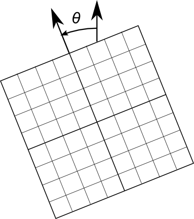
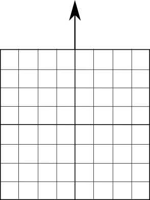
SIFT features are made up of histograms over 4x4 blocks. The standard SIFT feature uses a 4x4 grid of these blocks, sampling in total a 16x16 window. When applied to the base layer of a scale-space image stack, the pixel spacing in the sample window is the same as the spacing in the image stack, and no scaling is required -- only rotation and translation. As you climb the stack, the sample window will scale up at the same rate as scale-space.
Create a mapping that you can supply to your transformImage function that you created in Lab 2 to extract the image on the right, given the point structure and an image pyramid, following the template below:
% sample = extractSample(point,pyramid)
%
%   point - a point structure.
%
%   pyramid - a cell-array pyramid, pyramid{indLevel}(i,j,k) gives the pixel at
%             location i,j, scale plane k within the octave, and octave indLevel

% Author: Phileas Fogg
% Term: Winter 2012-2013
% Course: CS498 - Computer Vision
% Assignment: Lab 4 - SIFT feature description

function sample = extractSample(point,pyramid)
Test extractSample on a few feature points, using pyramidBlurred as the input pyramid. Do the image gradients look correct?
Compute SIFT feature descriptor
And now we come to the grand finale (of this lab)!
From the dIdx and dIdy image patches, compute the magnitude and angle images for the patch.
Be sure to add an offset to the angles in the rotated angle to account for the fact that dIdx and dIdy are still being measured in the coordinates of the original image. And to make the histogram process easier, after offsetting theta, map theta back into the range -pi to pi, or the range 0 to pi.
Computing the SIFT descriptors! (Lowe's SIFT paper has a good figure for this, the link is below.) In each 4x4 pixel block of the image, compute the 8-direction histogram of edge weights. Each pixel will contribute a weight proportional to its edge magnitude to a histogram. The contribution should also be weighted by a Gaussian distribution centered over the whole sample patch. You can create a weighted Gaussian disribution using createGaussianWeightingForFeatureSample.m. You do not need to use the bilinear weighting technique mentioned in the text and paper; an independent histogram in each block will be adequate for our purposes.
Concatenate the histograms from all the blocks. You can concatenate them in whatever order you like. This forms the 128-dimensional SIFT feature-vector.
Normalize the feature vector so that it sums to 1. (All the values in the feature vector should be positive.)
Set all values in the histogram that are greater than 0.2 to 0.2. Renormalize the histogram.
Create a method according to this template that computes the sift descriptor for a given sample point and derivative pyramids:
% point = extractDescriptor(point,dIdx,dIdy)
%
%  Computes the SIFT descriptor for a point.
%
%  dIdx - pyramid of x derivatives
%  dIdy - pyramid of y derivatives
%  point - the point structure.
%
%  Output:
%    point.descriptor - a vector of length 128 with the full SIFT descriptor for this point.
%

% Author: Phileas Fogg
% Term: Winter 2012-2013
% Course: CS498 - Computer Vision
% Assignment: Lab 4 - SIFT feature description

function point = extractDescriptor(point,dIdx,dIdy)
And finally, wrap up the descriptors for all the points:. You can add an empty descriptor field to all the points in a struct array of points using [results.points.descriptor] = deal([]); (and rmfield could be useful if you want to remove a field.)
% results = extractDescriptors(results)
%
%  Computes the descriptors for all the points.
%
%  results - the results structure
%    input:
%     whatever you want from the previous methods..
%
%    output:
%     results.points.feature

% Author: Phileas Fogg
% Term: Winter 2012-2013
% Course: CS498 - Computer Vision
% Assignment: Lab 4 - SIFT feature description

function results = extractDescriptors(results)
Now you can submit your labs and wait in suspense for next week's lab to see if they will give you good matches!
Fun Ideas
- We have skipped the bilinear interpolation during the computation of the histogram. This can increase your matching performance.
- The book mentions a variety of alternative features -- e.g. circular features that are said to slightly out-perform SIFT. You could also compute these... and test to see which is better next week.
- Do you have your own fun ideas that you would like to try?
References
- David Lowe's SIFT paper, available on his SIFT page
- Richard Szeliski's Computer Vision: Algorithms and Applications, (available on his Book page, and from booksellers everywhere...)
- Bilinear interpolation when computing histograms pp. 96-97/110
- 4.1 Points and Patches (includes High-level description of algorithm) pp. 192-194/216-219, 197-199/