Lab 2: Introduction to Filtering and Histograms

Overview

• Find edges using derivative filtering
• Explain why the edge filter's values should sum to 0
• Create and interpret edge magnitude and phase images
• Compute histograms of image intensities and angles

I will provide you with a printout of the lab checklist

Prelab

If you have not yet done so, install Matlab on your computer. It is available through a network install.

I will provide a printed copy of the lab checklist.

Deliverables

• A single Matlab file divided into cells (groups beginning with a two-percent %% comment), following this template.
• The image you worked with.
• Your m and theta images (either separately, or combined using showEdgeImage)
• The cropped image you created an edge histogram of
• Your edge histogram
• (optional) Results images that you created with your program.

Useful Matlab commands for this lab

imread

Read a Matlab image. e.g. I = imread('filename.png');

imshow

Show an image; open a new figure to hold the image if needed. e.g. imshow(I)

shg

"Show graph"; Bring the current figure window to the front. e.g. shg

size

Find the size of a Matlab array. e.g. sz = size(I);

zeros

Make an array of zeros with a specified size. e.g. black = zeros(sz);

ones

Make an array of ones with a specified size. e.g. white = 255*ones(sz);

ginput

Allow user to click points on a graph. e.g. [j,i] = ginput(1); will allow you to click on one (1) point on the graph. If you do not supply an argument, ginput will keep collecting points until you press the enter key.

imfilter

Filter an image using correlation. e.g. I2 = imfilter(I2, [-1 0 1]); is a simple derivative filter in the j direction.

normpdf

Create a Gaussian filter (or Probability Distribution Function -- PDF). e.g. blurFilter = normpdf(xrange,mu,sigma)

double

Convert an image to the double type. e.g. I = double(I)/255;

class

Find the type of an array. e.g. cls = class(I);

plot

Plot 2-d data. e.g. plot(x,y,'ro-'). If you use doc for help, be sure to check out the LineSpec link.

bar

Plot a bar graph. bar(h)

If you would like more information about any of these functions, use help functionname to get the command-line help. doc functioname brings up the full Matlab help browser for that function.

You may have noticed in the examples above, some commands end with a semi-colon, while others do not. This is because the semicolon is not required on statement endings. Matlab uses one line for each statement. (If you want to continue a statement over multiple lines, use ... at the end of each line except the last one.) The semi-colon is used for hiding the result of a statement. So if you want to hide the results of a Matlab statement (which you generally do if it is a HUGE image), put a semicolon at the end of the line. If you want to see the results printed to standard-out, leave the semicolon off. (In the examples above, the commands without semicolons don't have any output at all.)

This Matlab Tutorial from Brown University is very good. Everything discussed in the tutorial is essential to programming in Matlab¹. Although I try not to assume familiarity with Matlab in this lab, if this is your first time using Matlab, I encourage you to work through the tutorial in depth.

In particular, the tutorial has a section on working with images. Search for %(8) Working with (gray level) images. It's at the end.

Repeating Steps 1-4

Copy or re-do your steps 1-4 from lab1.m. Correct any errors in your graded Lab 1

5. Finding edges with a derivative filter

Filtering can also be used to find edges in an image. We will use a simple derivative filter to accomplish this task. A derivate filter is a discrete approximation of the partial derivatives of an image. Think of the grayscale image IGray as a function mapping row/column indices i and j to inensity values, e.g. IGray(i,j) as a continuous function. Then the partial derivatives of this function would also be images e.g ∂I/∂i (i,j) = I_i(i,j) gives the partial derivative in the vertical direction at each point in the image, and ∂I/∂j (i,j) = I_j gives the partial derivative in the horizontal direction.

While I might have been a continuous function somewhere in the camera that took the picture, all we have are discrete values. So instead of computing the "true" derivative, we will compute an approximation. The classic approximation of a derivative is I_i ≈ (I(i+di)-I(i))/di. Instead of this we will use I(i+1) - I(i-1). (This result will have half the magnitued of the true derivative, but that is not generally a concern for us. We are most interested in the relative values of the derivative from one spot in the image to another.)

Create a filter that will compute I(i+1) - I(i-1) for each point in the image. Run this filter on IGray in both the i and j directions, to create two images, one for dIdi and the other for dIdj.

I believe you will find it convenient to compute the derivatives with respect to i and j instead of x and y, since this is the coordinate frame used by Matlab (and many other programs) to store images.

In your template for this section, answer the question, "why is it important for the sum of the edge filter to be zero?"

Create two more images, where each pixel in the image is computed according to

  m(i,j) = sqrt(Ii2(i,j) + Ij2(i,j));
  θ(i,j) = atan2(Ij(i,j),Ii(i,j))

(You do not need to use any loops to compute these images. One thing that is tricky about them is that Matlab interprets A*B and similarly A^b as matrix operations. To specify these to be done element-wise, use A.*B and A.^b instead.)

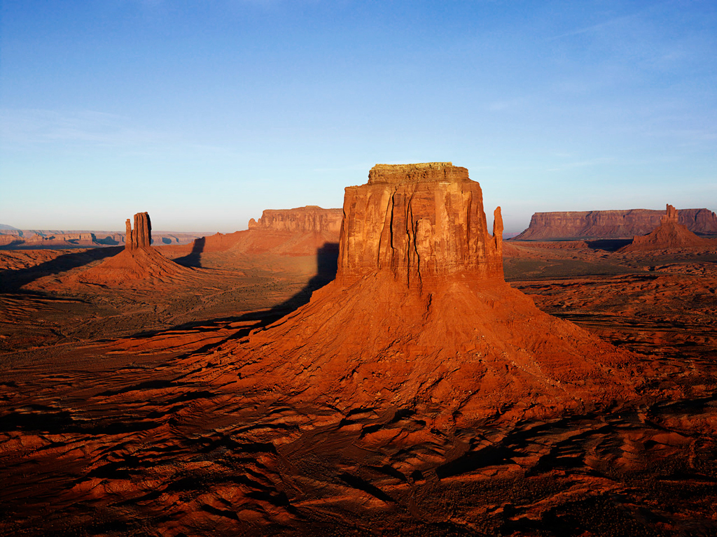
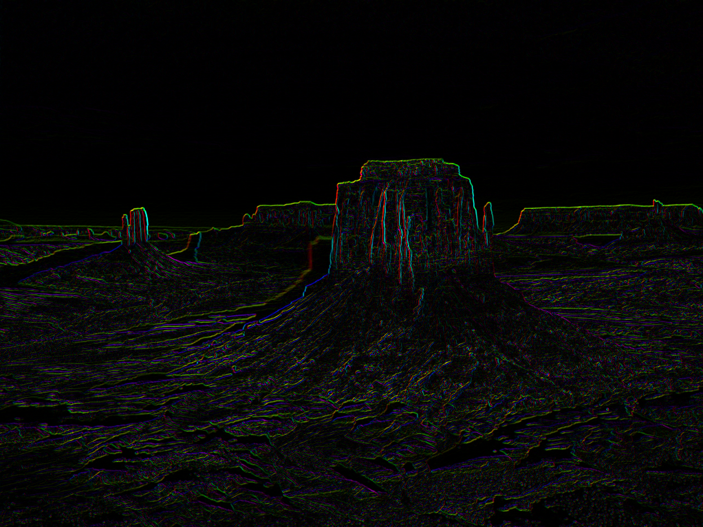
These images compute the magnitude and direction of the local slope of the image intensity function. You can view them separately using imshow, or view them together as a single color image using showEdgeImage(m,theta). showEdgeImage(m,theta) will produce an image that looks something like this: (starting from this stock Microsoft image — for your report, use your own image, not this one). The edges in the figure below use a different color convention than the provided showEdgeImage() uses

6. Histograms

In this part, we will make summary descriptions of gray-scale images. Set I to grayscale or replace I with the name of your grayscale image throughout the part that follows.

a. Image histogram

Histograms are often used to summarize an image. The simplest histogram is the count of each intensity in an image. Create a histogram of the image using a for-loop (there's not really a good way around this.). To iterate over all the pixels in the image, it can help to create a single-row version of the image. You can do this with IColumn = I(:)'. The bar command is useful for displaying a histogram. You may want to compare histograms for dark and light images, to see if the histogram does what you expect.

This is one of the few simple things that is very hard (if not impossible) to do with indexing of any kind in Matlab. You will need a loop.

b. Weighted edge histograms

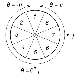
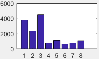
Pixel intensity histograms are good for summarizing the brightness of an image. If we want to summarize the shape of an image, a weighted edge histogram can be more useful. Let's return to the small image you cropped out earlier. Suppose you crop out the same portion of the m and θ images. Now compute a histogram of the θ directions, but instead of adding 1 into the bin, add the value of m. Use eight (8) directions, and make sure that theta falls in one of those eight directions. By default, θ is in the range -π to π. Can you map it into the range 1 to 8, as illustrated in the figure below? (This figure uses the dIdi and dIdj images, so theta is measured from the i axis instead of the x axis.) What weights do you get for your histogram bins? Do they make sense? You can plot your histogram using the bar method.

Here is an example of what your edge image may look like: (Spring 2018: Updated images to match the ones shown at the start of the lab period)

Please include in your packet printouts of your cropped image, edge histogram, and diagram illustrating the edge boundaries (like the example images above).

Fun Ideas for Excellent Credit

For excellent credit, try some of the ideas below or your own. To get credit, your extra work should truly be excellent.

• Check out what you can accomplish with blurring and edge images with this lab from Brown University (You can find the best student submissions from the class homepage)
• You can downsample an image by selecting every other pixel along the rows and columns. Can you do a simple downsampling using Matlab's range operators? If you want to store your downsampled images in a single variable, a cell array might be useful. (Not to be confused with cells in a .m file, which are completely different.) Cell arrays are like matrices, except that they can hold any matlab object in each position. Try stack{1} = I;, imshow(stack{1});, etc.
• For more advanced downsampling, you can smooth the image before downsampling. Try downsampling an image of a picket fence or a striped shirt both with and without smoothing. Do you see aliasing in the unsmoothed image? (You may need to downsample multiple times to get the effect.)
• Can you create your own image by alternating black and white images between rows? (You can use the Matlab range operators and indexing for this, too.)
• Logical indexing is a powerfull alternative to range indexing. In a logical index, the index is an array the same size as the image (or as one dimension of the indexing). You can create a logical mask with an expresssion like mask = I > 0.5;, and then only edit the selected pixels with an expression like I(mask) = 0. What creative images can you come up with using masking? (If you want to use a mask on a binary image, you will need to duplicate it for each channel, e.g. [mask(:);mask(:);mask(:)])
• You can also create fun images using alpha-compositing. This is where you combine images together, but multiply them by an "alpha" mask first. What fun images can you come up with using an alpha mask? (How might you compute the mask automatically from the image? Or from some simple user input?)
• The gray-scale method we use in this class works well, but other weightings of the channels can give more pleasing results. Look up in the text the section on color, and try converting your image to gray-scale (or a different full 3-d color space like YCrCb). Does this make your grayscale image look better? Do you think using a color space closer to human perception would increase the performance of your computer vision algorithms? (You may want to revisit this question later in the quarter.)
• What would you like to do automatically from images? Give it a try!

The fine print

¹ Except you should use (1:10) instead of [1:10]. As the squiggly orange mlint line will tell you, brackets are unnecessary around a range. They imply a call to the concatenation function, so using parenthesis will save you a few clock cycles.