CS498
Lab 7
Deliverables
The lab checklist will be provided to you in hard-copy
Overview
In this lab, we get to put features to work! To do this we will...
- Compute the interest points and features for two images using a predefined method
- For each feature point in the right image, find the closest feature in the left image using a predefined method.
- Some of these matches will still be false. To further refine the matches, we will apply RANSAC to all the matches to find a consistent subset
- As in Lab 3, we will pad the left image with a black image of the same size on the right
- Finally, we will transform the right image to line up with the left image with black matte automatically. At the end of this lab, we will have a program that does Lab 4 completely automatically!
Useful Matlab commands for this lab
These methods work best on images no larger than about 810x1080
- detectSURFFeatures
- Given an image, find the locations of interesting points in it.
points = detectSURFFeatures(grayImage) - extractFeatures
- Given interesting locations, extract features where possible.
[features, validPoints] = extractFeatures(grayImage,points) - matchFeatures
- Given features from two images, find the indices of the features which match between the two images.
[indexPairs, matchMetric] = matchFeatures(features1, features2)For the ith match, indexPairs(i,1) gives the index of a feature in features1, and indexPairs(i,2) gives the index of a feature in features2 - showMatchedFeatures
- Displays the matched featuers.
detectSURFFeatures(I1, I2, matchedPoints1, matchedPoints2). You must provide this method with two arrays of feature-points of the same size, with matchedPoints1(i) being a point in the first image corresponding to matchedPoints2(i) being a point in the second image. - estimateGeometricTransform
- Given matched points, with possible false matches, find a transform from one image to another.
tform = estimateGeometricTransform(matchedPoints1,matchedPoints2,'projective');Note that tform.T is the transpose of the homographic transform we discussed earlier. - imwarp
- Warp one image onto another.
IWarped = imwarp(I1,tform,'OutputView',imref2d(size(I2)));In this example, the 'OutputView' option with valueimref2d(size(I2))specifies to create an image the same size as I2, and to use the coordinate system of I2 in the resulting image.
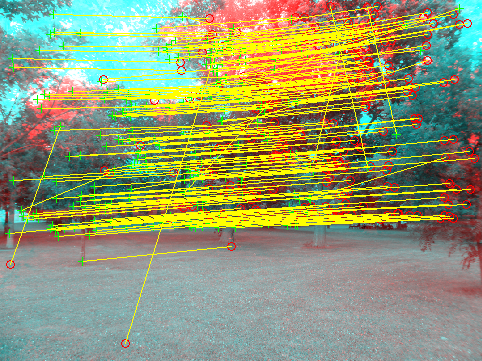
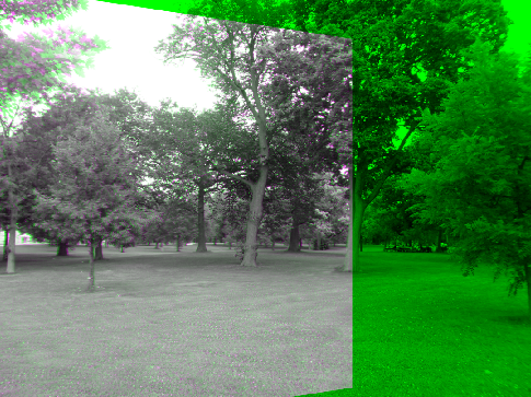
Create an image with the matches, and a stiched image like the ones below, and submit them with your results!
Please note that the example images map the left one onto the right, but you should map the right onto the left so that you can pad the left image on the right with a black matting as described above
matches.png
composite.png
Fun Ideas
- Try creating a chain of images, by finding the homography between each image and the next, then mapping all of the images back into the plane of the original image.
- Test your tranform under a variety of conditions... does it work if you turn one image upside-down? Does it work if you scale an image by a factor of 2? How about for a factor of 1.5? What other conditions could you try?
- Although we have developed this algorithm to work on two images using a homography mapping between them, it can find matches between images with some projective distortion -- as long as there are enough co-planar features in the image. Try running the algorithm on two images taken from slightly different perspectives.
- Use Adaptive non-maximal suppression (ANMS) to find interest-points in lower-contrast regions of the image (e.g. the grass in the images above). See the text, Section 4.1.1, Figure 4.9, pp. 191/
- Solving the over-constrained set of linear equations does not find the best transform. Once you have the transform, refine it using a gradient descent method.
- Can you reproduce a plot something like Figure 11 in Lowe 2004? It wont' look as clean if it is based on just matching two images, but does it show the same general trend? (You could consider inliers from your final results to be "true positives" and the rest to be "false positives", or you could apply a known transformation to an image as Lowe and 2004. Then you know how the points should transform from one image to another, and don't need to use RANSAC.)
- Do one of the excellent-credit activites suggested in last-week's lab
- Do you have your own fun ideas that you would like to try?
Porject / Undergraduate Research Ideas — Can you think of a minute step toward this goal?
- The book mentions a variety of alternative features -- e.g. circular features that are said to slightly out-perform SIFT. You could also compute these... and test to see which is better.
- Using epipolar geometry, you can find a mapping between any two images that constrains the images to be along a line. You could implement this mapping, and use the RANSAC approach to find an epipolar match between two images. This would allow you to find more corresponding points between any images of 3D scenes, but it might be harder to filter the false-positives, because any two points along the epipolar line would be allowed to match, even if they are false matches. It also may take longer to run RANSAC, because you will need to find more than 4 point correspondences to compute the initial estimte of the epipolar constraint.
- Now is the time where you can REALLY go to town with your Google street-view approach! Or you could try to convince Google to map our campus! (I think you would need to contact HR first...)
References
- David Lowe's SIFT paper, available on his SIFT page
- Richard Szeliski's Computer Vision: Algorithms and Applications, (available on his Book page, and from booksellers everywhere...)
- Bilinear interpolation when computing histograms pp. 96-97/110
- 4.1 Points and Patches (includes High-level description of algorithm) pp. 192-194/216-219, 197-199/
- RANSAC 6.1.4 (p.281-282/)