CS498: Computer Vision

CS498

Lab 3

Deliverables

The checklist will be given to you in hard-copy. If printing your own copy, you may only want to print the first page, but read the second page online.

createFilters.m
filterStack.m
findDiffOfGaussianStack.m
findGoodExtrema.m
findFeaturePoints.m (optional)
sift.m (your top-level script)
Answers to these questions
- How does the SIFT interest-point detection achieve illumination invariance?
- How does the SIFT interest-point detection achieve rotation invariance?
- How does the SIFT interest-point detection achieve scale invariance?

Overview

In this lab, you will perform a few steps to produce a difference-of-Gaussian stack, and extract multi-scale interest points from that stack.

Convert the image to gray-scale by averaging the R, G, and B channels as in Lab 1.
Sucessively filter the image with larger and larger Gaussian filters to produce different levels in a scale space.
Subtract the layers of the stack to produce Difference-of-Gaussian (DoG) images.
Find extrema (minimum and maximum values) in the Difference of Gaussian images.
Filter the extrema based upon the intensity value of the DoG image at the extrema location.
Compute the Hessian -- the second derivatives of the image in the x and y directions -- for all of the difference of Gaussian images
Finding interest-points using the Hessian, as discussed in text in the section on the SIFT filter.
Filter the extrema based upon the eigenvalues of the Hessian at the Difference-of-Gaussian location.
(optional) Successively down-sample the image to produce an image pyramid, repeating the steps above for each layer.
Convert pixel locations and sizes in the reduced-size images to pixel locations and sizes in the original image.

Useful Matlab commands for this lab

normpdf: Create a Gaussian filter (or Probability Distribution Function -- PDF). e.g. blurFilter = normpdf(x,mu,sigma)
imfilter: Filter an image. e.g. IBlurred = imfilter(I, h, 'replicate')
dbstop if error: Stop if an error occurs.
dbclear if error: Don't stop if an error occurs.
dbquit: exit debugging mode
dbup: Go up a level in the call stack
dbdown: Go down a level in the call stack
size: Find the size of all or the given dimension of a matrix. e.g. size(stack) could return [400,300,5] and size(stack,2) would return 300
length: Return size of first non-singleton dimension. e.g., if size(A) is [1 7 5], length(A) returns 7. This is meant to be used with column and row vectors which have only one dimension greater than 1
find: Find the non-zero entries. e.g. x = [0 0 0 0; 0 0 1 0; 1 0 0 0]; indices = find(x); returns indices = [2 6], the i index of both points if i keeps counting throughout the array
ind2sub: [ii,jj,kk] = ind2sub(size(x),indices) returns the actual ii, jj, and kk indices in the original matrix: ii = [2 1]; jj = [1 3];
reshape: Restore the shape of a flattened matrix. e.g., x = reshape(x(:),size(x)) flattens and then restores x to its original shape.
sub2ind: indices = sub2ind([ii,jj,kk]), gives the same result as the find example above.
[a,b;c,d]: Concatenate the matrices a,b, c, and d into a larger matrix.

Matlab's cell arrays

A cell array is like a Matlab array (or matrix), but it can store any Matlab object in it. To create a cell array x, you can use x = {};, or you can simply assign a value in an array, x{1,3} = [1 2 3 4 5];.

In the example above, if we wanted to access the numbers 3 and 4, we could use x{1,3}(3:4). This multiple- or nested- indexing can come in handy!

For more information on cell arrays, see Mathworks' documentation of cell arrays.

Converting the image to gray-scale

Create a gray-scale version of the image, as in Lab1. This will be the "base image" for the first level of the stack.

Create a stack of filtered images

Without changing resolutions, we can consider multiple scales in an image by filtering the image with different Gaussian filters. As the standard deviation of the Gaussian filter grows larger, it removes more and more of the fine details, leaving only larger-scale features in the image. We will call these images with the same resolution, but different filtering scales an "image stack".

Scale-space is logarithmic. In a full pyramid, each successive level (octave) of the pyramid is half the size of the previous level, so the i^th layer is reduced by σ = 2^i-1. To find the layer from the sigma, we would use i = 1 + log₂ σ. This is why it is called a logarithmic scale. In practice, we don't use the logarithm, since we only need to compute the scale from the level in the pyramid or image stack. So you might want to think of scale-space as being exponential, instead!

In this lab, we will be detecting features at multiple scales, but only within two octaves (two powers of two). So the lowest level of our stack will have a scale factor of 1 (blurred with a Gaussian of σ = 1) and the highest layer will have a scale factor of about 4 (blurred with a Gaussian of σ = 4). To evenly space our stack layers in the log-scale of scale space, we will space them exponentially as well. Suppose we desire s scales per octave (that is, per power of two in scale space). Then the difference in scale between successive levels of the pyramid will be 2^1/s, and if two scales are i steps apart, then the difference between their scales will be 2^i/s.

As discussed in class, you can create a filter using a command like normpdf(xsamples,0,sigma), where you compute sigma using the 2^^... formula from the previous paragraph. You want to select the x samples so they are symmetric (e.g. [-2, -1, 0, 1, 2]), and with enough elements to include all the "important" elements of the filter. No matter how many samples you ask for, they will all be non-zero, but some will be very close to zero -- you don't need those. Exactly which ones are "close to zero" is something I want you to decide.

Write a method to create a cell-array of filters, where each filter will filter one level image stack. As in Lab 1, we will filter along each dimension individaully to speed up the filtering time. Your method should meet the specifications in this template: To save processing time, reduce the size of your filters so that the elements near zero are not used in the filtering. Make sure you re-normalize your filters so that they sum to one after dropping the smaller coefficients.

% h = createFilters(stackSize,s)
%
%   stackSize -- the number of layers to produce filters for (usually s + 3 2*s+1)
%   s -- the number of scale spaces levels per octave (usually 3)
%
%   h -- a cell array of row vectors.  h{i} is row vector representing the
%        Guassian filter for the i'th level of the image stack.
%
%   (stackSize should be three levels bigger than s to get sufficent overlap.)

% Author: Phileas Fogg
% Term: Winter 2012-2013
% Course: CS498 - Computer Vision
% Assignment: Lab 3 - SIFT interest-point detection

function h = createFilters(stackSize,s)

Once you have created these filters, you can apply them in both the horizontal and vertical direction, as discussed in class, to do efficient 2-D filtering. Write a method that creates a three-dimensional matrix stack, where each layer the matrix, stack(:,:,i), is a layer in the filter stack. Be sure to use an option like 'replicate' when creating the filter to avoid problems at the edge of an image.

% stack = filterStack(baseImage,h)
% 
%   Create a series of filtered images from a base image.
%
%      baseImage -- grayscale image as 2d matrix
%      h -- cell array of 1d row vectors
%
%   stack(:,:,i) contains the version of baseImage filtered with h{i}

% Author: Phileas Fogg
% Term: Winter 2012-2013
% Course: CS498 - Computer Vision
% Assignment: Lab 3 - SIFT interest-point detection

function stack = filterStack(baseImage,h)

Create the Difference of Gaussian (DoG) stack

To create a difference-of-Gaussian stack, all you need to do is subtract each layer from the layer following. Create a method that does this using this template:

%diff = findDiffOfGaussianStack(stack)
%
% Create Difference-of-Gaussian stack from stack of Gaussian images
%
%   stack - three-dimensional array, where stack(:,:,i) is a  
%           gaussian-filtered image.
%
%   diff - the difference-of-gaussian stack.
%
% See filterStack -- creates stack of Gaussian images

% Author: Phileas Fogg
% Term: Winter 2012-2013
% Course: CS498 - Computer Vision
% Assignment: Lab 3 - SIFT interest-point detection

function diff = findDiffOfGaussianStack(stack)

Find interest-points and filter based on intensity

You may want to develop this next method as a script, and then convert it to a method once it is working. This allows all your local variables to be in the workspace, and if an error occurs, you can see what their values are at the time of an error. An alternative method is to use the Matlab commands dbstop if error and dbclear if error to enable/disable going into debug mode when an error occurs. See other useful commands for debugging in the table at the start of the lab.

The interest-points are simply the minima and maxima of the DoG stack. In particular, these are the points that are either greater than or smaller than the 26 points that are nearest neighbors both in the image plane around them, and in the plane above and below. (See the figure in the text.) The function imregionalmax can be used to find the maxima that meet this criteria: maxStack = imregionalmax(diff);. To find the minima simply run imregionalmax on the image -diff. This function returns a logical image, that is, an image where all values are "true" or "false". The "true" values in this image mark the locations of the maxima. Be sure not to accept any points at the edges of the image, or in the top or bottom images of the stack. imregionalmax will return this.

Remove the points that have a value of less than 0.03 in the DoG stack. (This assumes that you have scaled the original pixel values to be in the range [0 1] instead of [0 255].)

Wrap up your point-finding code into a matlab function following this template:

% [ii,jj,kk] = findGoodExtrema(diff)
%
%  diff -- the DoG image
%  
%  ii -- a list if i-indexes for the interest points, in the dimensions
%        of this stack
%  jj -- similarly
%  kk -- the depth index of interest points in this stack.
%        (This gives the level of the point, and can be used to find the scale of the point.)

% Author: Phileas Fogg
% Term: Winter 2012-2013
% Course: CS498 - Computer Vision
% Assignment: Lab 3 - SIFT interest-point detection

function [ii,jj,kk] = findGoodExtrema(diff)

For debug purposes, you can view a projection through the whole stack by using the method imshow(max(maxStack,[],3))

Both this and the previous section can be accomplished with indexing and logical arrays to avoid loops, although there will still be some loops needed.

Displaying your points

At this point, display your images using the displayPoints function, which displays circles of the specified size at the specified location in the image. Use help displayPoints to see usage and an example of how to use this method with ii, jj, and kk. (You can also see an example of how to create the structure this method accepts as an alternative, which could be helpful if you want to implement the full pyramid. Feel free to put additional fields into the structure for your own purposes. In my implementation, I store s and the filter stack in the structure, just for debugging reference.)

Take a screenshot of your Matlab figure and save it as points.png.

If you would like to display an individual point, I can provide you with code. Please ask.

Matlab's structs (purely optional)

A matlab struct is essentially an object with public member variables. You can create a structure by simply assigning to the member variables. To create a structure s with member variable x, you can use s.x = 'anything you want';. You can also create a new struct with s = struct();

For more information on structs, see Mathworks' documentation of structs

You don't need to use cell arrays to hold structs. The normal array syntax works just fine with structs. For example, to create an array of points, you could use

point.i = 1;
point.j = 5;
points(1) = point;
point.i = 4;
point.j = 3;
points(2) = point;

You can access the points in multiple ways

point = points(i);
disp(point.x)

disp(points(i).x)

For more information on struct arrays vs. cell arrays, see Mathworks' documentation of this topic.

Produce an image pyramid (purely optional)

So far, we have found interest points in the lowest level of the image pyramid. You could just use larger and larger filters to continue to higher scales, but filtering with a large filter can take a long time. So to avoid that, we wil create a pyramid of images.

Our (optional) final pyramid will be built of multiple image stacks at successively smaller resolutions. Building the image stack is important for matching features at widely-varying scales.

Create three one-dimensional cell arrays. For all of these cell arrays, the contents of the cell array will represent a level in the image pyramid. The first cell array, pyramidBase, will contain the base image for each level of the pyramid. pyramidBase{1} will be the original image. For the remaining levels, you will take the base image from the previous level of the pyramid. The second cell array is pyramidBlurred. pyramidBlurred{i} will contain the pyramid stack of blurred Gaussian images for level i of the pyramid. The third cell array is pyramidDiff. pyramidDiff{i} will contain the DoG stack for level i of the pyramid. To find the base image for the levels beyond 1, take the image from the stack that corresponds to a blurring with a sigma value of 2. (Note that this is not the last image in the stack.)

You may notice that we are blurring an image twice -- once in the lower level of the pyramid, and again at the next level (e.g. with a sigma of 1 for the first image in that level.) This will slightly increase the blurring of the image, but you can neglect it.

Once you have pyramidBlurred, you can commpute the interest points exactly as we did at the lowest level. The only challenge that remains (other than debugging...) is converting the points you find back into indexes and sigmas that you can use at the lowest level. Consider how you have constructed the images, and what the effective scale of the filters would be if they were applied to the original unscaled images. Since a DoG layer technically has two scales, you can assign the scale as the larger, smaller, or geometric mean of these. As long as you use the same approach throughout, it should not affect your matching results.

Once you are satisified with this level, wrap it up into a method following this template:

%results = findFeaturePoints(I)
% 
% I - the input color image as a 3D array of type uint8 and range [0-255]
%
% results - A structure representing the extracted features and possibly
%           intermediate results
%     results.I -- the original 
%     results.points -- A one-dimensional struct array of points
%        results.points(ind).i -- the i-index of the ind point in the image plane
%        results.points(ind).j -- the j-index
%        results.points(ind).sigma -- the standard devation of the blur
%           applied to the point the image was extracted.
%
%         A bunch of other fields are not needed for this lab, but we will use them in the next lab:
%     results.s -- The number of scale-space levels per octave (not the same as the number of levels
%                  in a stack)
%     results.pyramidBlurred{ind} -- The blurred pyramid.
%     results.points
%        results.points(ind).iPyr -- the i-index in the pyramid stack where the feature was detected.
%        results.points(ind).jPyr -- the j-index in the pyramid stack where the feature was detected.
%        results.points(ind).kPyr -- the k-index in the pyramid stack where the feature was detected.
%        results.points(ind).indLevel -- the level in the pyramid where the feature was detected
%           You could find the original point again using
%               results.pyramidBlurred{indLevel}(iPyr,jPyr,kPyr)
%                               
%     results may contain other fields for debugging purposes.

% Author: Phileas Fogg
% Term: Winter 2012-2013
% Course: CS498 - Computer Vision
% Assignment: Lab 3 - SIFT interest-point detection

function results = findFeaturePoints(I)

You might create a top-level script just to test this:

I = imread('Desert.jpg');
results = findFeaturePoints(I);
displayPoints(results);

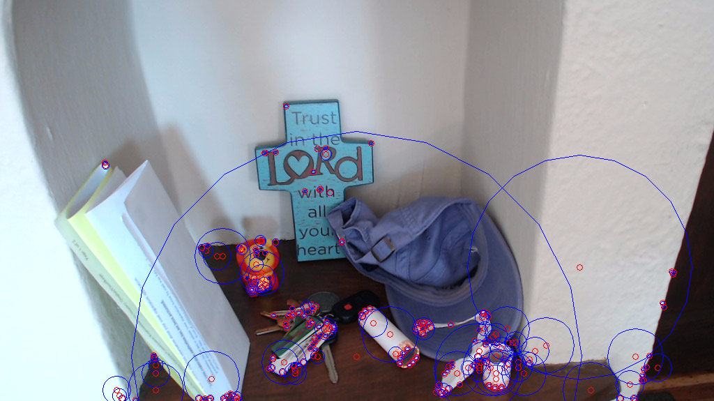
Hopefully you see something like the picture below. if the points do not appear on interesting points in the image, it's debugging time!

Fun Ideas

(As above) create a pyramid of images, with each level half the resolution of the one before, finding interest-points up to a scale as large as the whole image. Comment on why this is only O(log N) or so times the work rather than O(n) times the original work, where n is the size of the image.
Increase the size of the original image by a factor of two, filling in the new pixels with bilinear interpolation. This can increase the number of interest-points you find, if your original image has VERY detailed features (megapixel images will not benefit from this)
Locate pixels with sub-pixel accuracy. This can improve matching results. See the text (or the paper) for strategy.
If you are bothered by the multiple filtering not giving an exact Gaussian blur with the correct sigma (like I was), figure out the ideal Gaussian blurring so that two consecutive blurrings gives you the desired sigma. What is the difference in the sigma values? Does the problem accumulate and grow much worse as we go to sucessively larger levels in the stack?
Implement a multi-scale Harris point detector. The text says this finds different interest-points than the SIFT interest-points, that are also good, increasing the number of interest points available.
Szeliski mentions in the text that SIFT tends to find many features in high-contrast areas of the image, but fewer features in lower ones. He (and colleagues) suggest adaptively selecting points based on how close the nearest neighbor is. This is described in our text (see references below) and in a paper he wrote with Brown. You can ask me for a copy.
Do you have your own fun ideas that you would like to try?

References

Jimmy Huff's SIFT tutorial (with some simplifications by me)
David Lowe's SIFT paper, available on his SIFT page
Richard Szeliski's Computer Vision: Algorithms and Applications, (available on his Book page, and from booksellers everywhere...)
- Bilinear interpolation when computing histograms pp. 96-97/110
- 4.1 Points and Patches (includes High-level description of algorithm) pp. 192-194/216-219, 197-199/

Lab 3: Interest-point detection