CS498: Computer Vision

CS498

Lab 6

Prelab

The lab checklist is now posted and will be provided in hard-copy

An esubmit page is again available if you do not wish to print out your lab. As with the previous lab, exactly one PDF should be submitted.

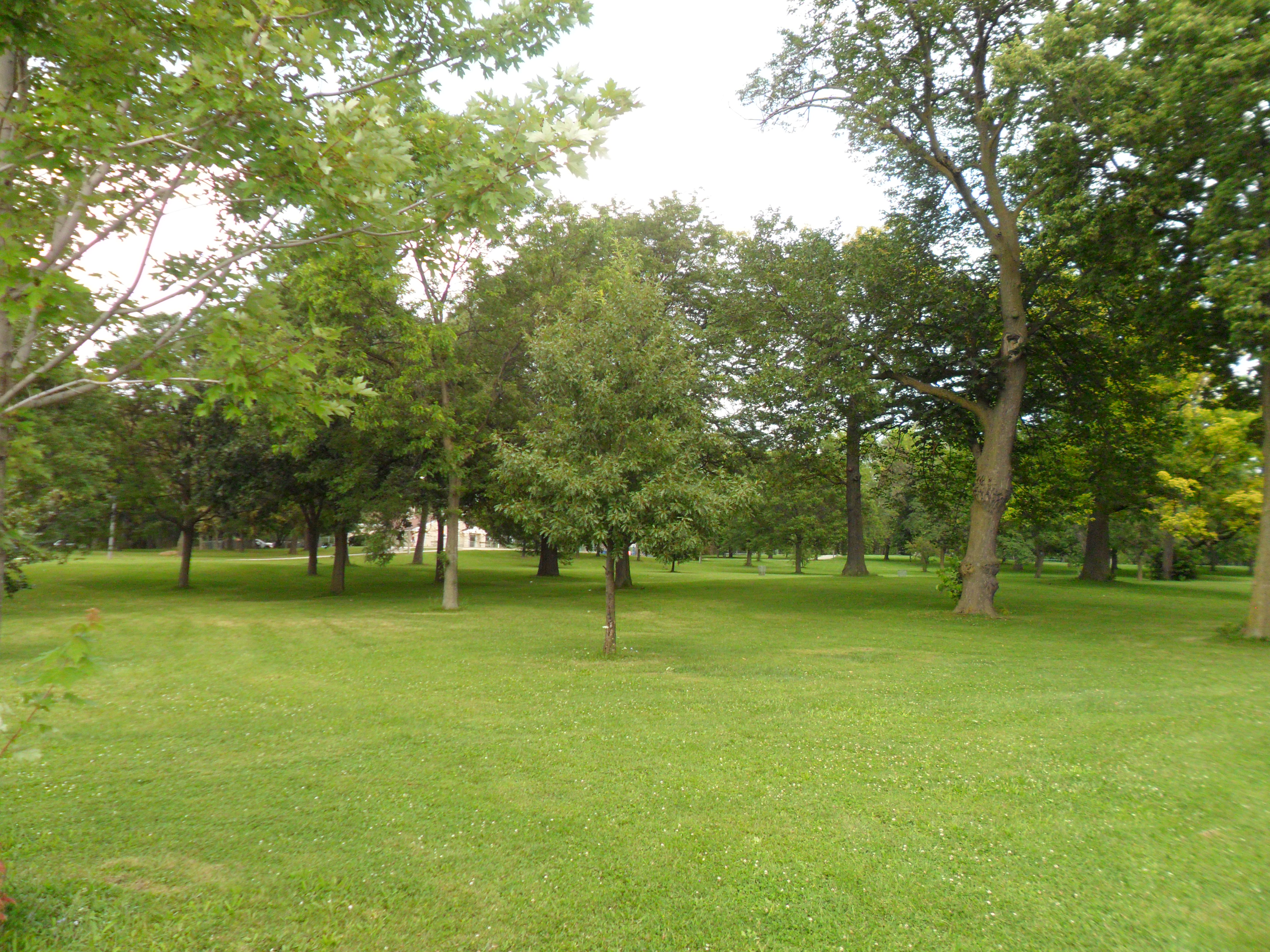
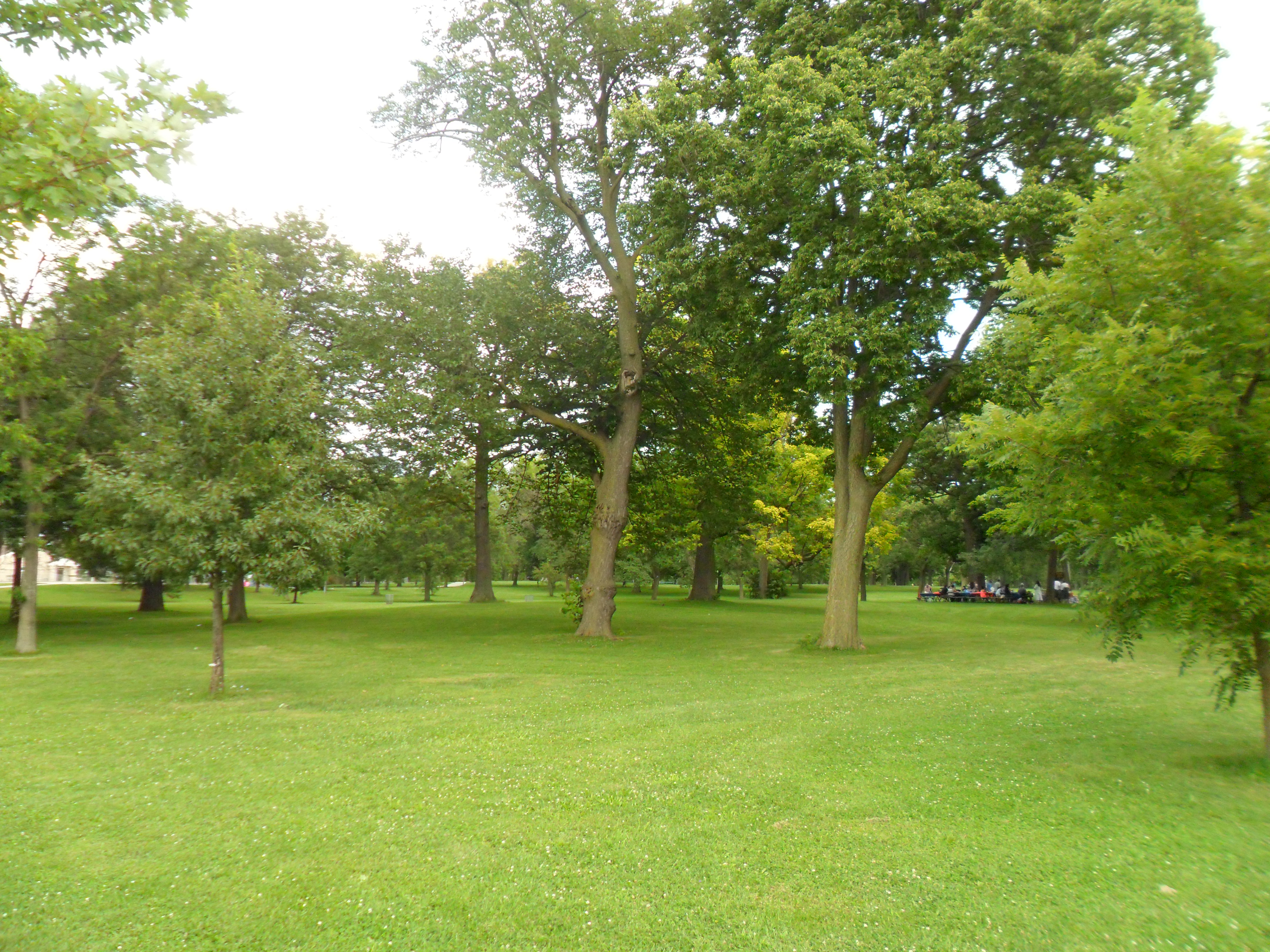
Before lab, take two pictures, with the camera lense at the same position, but pointing in slightly different directions. Try get at least a 50-80% overlap between the images. It is best if you take the pictures in a large area, since this will reduce the difficulties coming from taking a picture from multiple positions. Here is an example, although do be sure to take some pictures with more overlap than this. (They will be useful in later labs.)

A key concept for this lab is that two pictures taken from the exact same position only have image-based warping between them, not any 3D effects. In some sense, what the camera sees when it rotates around its center is a large flat image. We can map between any two images taken from the same position using a full 8-DOF homography, the same transform we can use to map a picture of a flat object from one camera view to another. In this lab, we will stitch two pictures taken from a single point of view together by finding a homography between the two pictures.

Many cameras today have multi-megapixel images. In their uncompressed form, these images are very large. Since we usually maintain several copies of an image in matlab, this can easily fill your computer's memory. I recommend reducing the size of these images until Matlab does not warn you that they are too large to display on your screen when you run imshow

Deliverables

In all your source files, be sure to include your name and the quarter (e.g. Winter 2012-2013.) And, in the templates you copy from below, be sure to edit the author block that follows the help block so that it is accurate for you.

Useful Matlab commands for this lab

ndgrid: Create a set of n-dimensional grids with the values of the index for each point in the grid. e.g. [ii,jj,kk] = ndgrid(1:2,1:3,1:4);
hold on: Keep the currents contents of a graph. The next plot will be plotted on top. e.g. hold on
hold off: Opposite of hold on.
plot: Plot 2-d data. e.g. plot(jj,ii,'ro-'). If you use doc for help, be sure to check out the LineSpec link.
imfuse: Overlay two images with 0.5 alpha compositing. e.g. IFused = imfuse(I1,I2,'blend');
size: Find the size of all or the given dimension of a matrix. e.g. size(stack) could return [400,300,5] and size(stack,2) would return 300
length: Return size of first non-singleton dimension. e.g., if size(A) is [1 7 5], length(A) returns 7. This is meant to be used with column and row vectors which have only one dimension greater than 1
x(:): Flatten a matrix to a column vector. e.g., col = H(:) flattens the matrix H into a 9x1 matrix
reshape: Restore the shape of a flattened matrix. e.g., x = reshape(x(:),size(x)) flattens and then restores x to its original shape.
*: Matrix multiplication can be used to duplicate rows or columns. For example, x * ones(1,5) produces five duplicates of the column vector x
repmat: An alternative to the matrix multiplication approach on the previous line. I've found it to be slower in practice.
[a,b;c,d]: Concatenate the matrices a,b, c, and d into a larger matrix.

Homographic point transforms

In Lab 4, we looked at computing transformations with rotations, translations, and scaling. In this lab, we will look at two more effects: affine transformations and scaling.

Create a transformation which has the form

 [~i]   [a b 0] [i]
 [~j] = [c d 0] [j]
 [~w]   [0 0 1] [1]

which is not simply a rotation + a scaling.

Apply your transformation to the grid of points that you used in Lab 4

Rotation and scaling has two degrees of freedom (s and theta). Can you get a sense for how the remaining two degrees of freedom disort the image?

Now add a tiny number (on the order of 0.01 or 0.001) to one or both of the zero elements in the bottom row, e.g.

 [~i]   [a b c] [i]
 [~j] = [d e f] [j]
 [~w]   [0.001 0.01 1] [1]

We now have a homography matrix with eight degrees of freedom. (Even if we gave a value to the 1 in the bottom-right corner, it would not increase the degrees of freedom, since it gets divided out when we normalize the homogeneous point [~i, ~j, ~w] by dividing by ~w).

Apply your homography to the grid of points, dividing the i and j rows by the w row to compute true pixel values before plotting. Can you get a sense for how the elements in the last row impact the image?

Transforming the image

Use your transformImage function from Lab4 to apply your two homographies from the previous section to an image.

Marking correspondences in an image

Now that we have explored the homographic transformation, we will stitch two images using a full homography instead of just a translation like we used in Lab 4. This fuller transform will provide a cleaner alignment between the two images, at least when we use many correspondences to find it.

You can use your correspondences from Lab 4, or repeat these steps to find new correspondences.

Using ginput, mark four points on the first image. Mark the corresponding points in the second image. That is, mark four distinct points on objects in the first image, and mark the same points on the objects in the second image. Choose points that you can identify well, such as corners. Choose points that are widely spaced in the image so that your program does not have to extrapolate beyond them too much.

Save the points you use somewhere in your source code, so you don't have to remark the points every time you run the program. This should not be hard-coded in one of your matlab functions, but it could be hard-coded into your top-level script.

Finding the homography from the correspondences

In class , we discussed a technique for solving a linear system of equations to find a homography from one point-set to another. Apply this technique as follows

Create a method, makeASmall that creates two rows of the A matrix. As in section 6.1.3 (p. 279/) of the book, this is

A_small = [i j 1 0 0 0 -i₂i -i₂j]
    [0 0 0 i j 1 -j₂i -j₂j]

where i and j are the coordinates in the source image and i₂ and j₂ are the coordinates in destination image.

Use this header for the makeASmall method

% ASmall = makeASmall(i1,j1,i2,j2)
% 
% i1, j1 -- the indices in the first image
% i2, j2 -- the indices in the second image
%
% A -- Two rows of the A matrix used to solve for the Homography matrix,
%         representing a single point correspondence.
%

% Author: Phileas Fogg
% Term: Winter 2012-2013
% Course: CS498 - Computer Vision
% Assignment: Lab 6 - Homographic image warping

function ASmall = makeASmall(i1,j1,i2,j2)

Create a method that forms the full A matrix by concatenating all of the A_small matrices for the four point correspondences to form the full A matrix. There should be 2*n rows, where n is the number of correspondences you use (n=4 is the minimum you will need).

% bigA = makeA(matches)
% 
% matches -- a matrix where each row represents the indices of a match,
%            [i1 j2 i2 j2]
%
% bigA -- the full A matrix which is used to solve for the Homography matrix,
%         including all point correspondences.

% Author: Phileas Fogg
% Term: Winter 2012-2013
% Course: CS498 - Computer Vision
% Assignment: Lab 6 - Homographic image warping

function bigA = makeA(matches)

Create a method that creates the full b column vector. This vector is the concatenation of the b_small vectors for each pair of corresponding points, where b_small is ...

b_small = [i₂-i]
    [j₂-j]

Use this header for the makeB method

% bigB = makeB(matches)
%
% matches -- a matrix where each row represents the indices of a match,
%            [i1 j2 i2 j2]
%
% bigB -- the full B matrix with used to solve for the Homography matrix,
%         including all point correspondences.

% Author: Phileas Fogg
% Term: Winter 2012-2013
% Course: CS498 - Computer Vision
% Assignment: Lab 6 - Homographic image warping

function bigB = makeB(matches)

Concatenate a stack of B_small matrices to form the B matrix

Solve B = A*linearH for linearH.

You will use findTransform in some of the following labs, so be sure to write it so that it can accept more than four points. With more than four points, the problem is over-constrained, but the best solution to A linearH = b is a good first-level approximation to find the best point matches. If you use linearH = A\b to solve the system of equations, Matlab will automatically find the best solution under the hood.

Reshape linearH into a square matrix. Indexed-assignment can help here. But be aware that Matlab counts along columns, whereas the linearH matrix is indexed along the rows. Also note the 1's in the definition of H that are not included in linearH.

Wrap all of the above into another method, findTransform, which conforms to the following heading:

% H = findTransform(matches)
%
% matches -- list of matches in rows of [i1 j1 i2 j2]
%
% H -- transformation [i2,j2,w2]' = H*[i1,j1,1]'

% Author: Phileas Fogg
% Term: Winter 2012-2013
% Course: CS498 - Computer Vision
% Assignment: Lab 6 - Homographic image warping

function H = findTransform(matches)

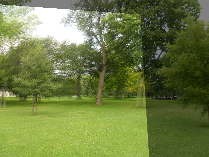
Now you can use your image transformation techniques from the first section to map one image onto another!

After fusing your two images, you should have something like this:

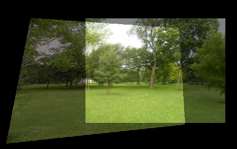
One of the fun ideas below is to modify things a bit so you get a black matted margin around the destination image:

Fun Ideas

Try creating a black mapped area around the image, as shown in the second image above. You can either modify the transform to go from the larger image, or modify your transforming function to accept an "offset" for the origin of the image, which is taken into account before transforming.
Use bilinear interpolation instead of rounding to the nearest pixel. This gives a smoother image when you enlarge.
In game engines, "mip-maps" or image pyramids are used to avoid aliasing when shrinking an image. Try building a pyramid of down-sampled smoothed images, and automatically selecting the scale based on how many pixels the destination image pixel would cover when mapped back onto the source. (Perhaps you can reproduce these images "from scratch.")
Try stitching several images in a row, either using homographies or panographies (6.1.2, p. 277/)
The imfuse approach we take here causes the images to be darker where they don't overlap. Can you make the images have full brightness like Figure 6.5. (p. 278/) by creating your own alpha-mapping strategy? You can create a mask for the transformed image(s) by transforming an all-ones image using the same mapping function
Can you build an entire panorama, going full-circle around a point? You may want to project the images on the the surface of a cube. Could you find the homography to go from one cube surface to the next? This would probably require some full 3-D camera geometry.
Google Street-view is built as a sequence of panoramas, centered at distinct points on a street. Can you build a simple "street view" of a pretty spot on campus?
Do you have your own fun ideas that you would like to try?

Readings

Szeliski (2011) Section 6.1 - 6.1.4 (pp. 275-280/)

Lab 6: Homographic image warping